fit_EOS

This code fits Birch-Murnaghan, Vinet, and polynomial log-log functional forms to Pressure-Volume (\(P\text{-}V\)) data provided by the user. The code uses libraries from python such as curve_fit from scipy.optimize in combination with InterpolatedUnivariateSpline from scipy.interpolate. The code supports error bars \(\delta P_i\) for the pressures \(P_i\), which changes the weights in the fitting process to \(w_i=1/\delta P_i\). It also supports error bars \(\delta V_i\) in the volumes \(V_i\) and propagates the errors accordingly for the fits. The output provides the fitting parameters for each of the functional forms with their respective errors from the covariance matrix. Different indicators for the resulting errors are provided to determine which fit worked better, including RMSE, standard deviation of the residuals, \(R^2\), and \(\chi^2\) (see below).

Download the code

Attention

⬇️ Get the code

📦 Download from GitHub

Fitting Equations of State using Vinet / Birch-Murnaghan / log-log to P-V data

Birch-Murnhagan EOS

The Birch-Murnaghan EOS of 3rd order is given by

\[ P (V)= \frac{3}{2} K_0 \left(\left(\frac{V_0}{V}\right)^{7/3} - \left(\frac{V_0}{V}\right)^{5/3}\right) \left(1 + \frac{3}{4}\left(K_0'-4\right)\left(\left(\frac{V_0}{V}\right)^{2/3}-1\right)\right)\]

and the Birch-Murnhagan EOS of 4th order is given by

\[ P (V)= \frac{3}{2} K_0 \left[\left(\frac{V_0}{V}\right)^{7/3} - \left(\frac{V_0}{V}\right)^{5/3}\right] \left[1 + \frac{3}{4}\left(K_0'-4\right)\left(\left(\frac{V_0}{V}\right)^{2/3}-1\right) + \frac{1}{24}\left(9{K_0'}^2-63K_0'+9K_0K_0''+143\right)\left(\left(\frac{V_0}{V}\right)^{2/3}-1\right)^2\right],\]

where \(K_0\equiv K(V_0)\), \(K_0'\equiv K'(P=0)\), and \(K_0'' \equiv K''(P=0)\), with \(K'(P)\equiv \left(\frac{\partial K}{\partial P}\right)\) and \(K''(P)\equiv \left(\frac{\partial^2 K}{\partial P^2}\right)\). Note that the derivatives are taken with respect to pressure, not volume. In fact, \(K'(P)= -K'(V)V/K(V)\). Further reading:

• Katsura, Tomoo, and Yoshinori Tange. “A simple derivation of the Birch–Murnaghan equations of state (EOSs) and comparison with EOSs derived from other definitions of finite strain.” Minerals 9.12 (2019): 745.

The normalized pressure EOS: \(F-f\)

Since pressure can be written in terms of the finite strain \(f\),

\[P=3K_0 f(1+2f)^{5/2}(1+2\xi f+4\zeta f^2+...),\]

where \(f= \frac{1}{2}( (V_0/V)^{2/3} -1 )\) is the Eulerian strain, the normalized pressure, \(F\) (not to be confused with Helmhotz free energy), is a simple linear or quadratic function of the strain,

\[F(f)=\frac{P}{3f(1+2f)^{5/2}}=K_0 (1+2\xi f+4\zeta f^2+...),\]

where \(\xi=(3/4)(K_0'-4)\) and \(\zeta=(3/8)[K_0K_0''+K_0'(K_0'-7)+143/9]\). A simple (weighted) linear fit to \(F(f)\) is equivalent to a third-order Birch-Murnaghan EOS, but it may be more precise and convinient because the intercept is \(K_0\) and slope is proportional to \(K_0'\). Further reading:

• Raymond Jeanloz. “Finite‐strain equation of state for high‐pressure phases.” Geophysical Research Letters 8.12 (1981): 1219-1222.

• Dion Heinz and Raymond Jeanloz. “The equation of state of the gold calibration standard.” Journal of applied physics 55.4 (1984): 885-893.

Tip

The code presented here is meant to fit \(T>0\) isotherms (where \(P(V_0)>0\)) and it can deal with either volumes in ų (\(V\)) or normalized volumes (\(V/V_0\)) as arguments. If the volumes are NOT normalized (they are not between 0 and 1), the code will divide the volumes by \(V_0={\rm max}(V)\) and shift down the values of \(P\) by \(P_{\rm shift}={\rm min}(P)\), such that \(P_{th}\equiv P-P_{\rm shift}\) looks like a zero-Kelvin isotherm that satisfies \(P_{th}(V_0) = 0\) by definition. Therefore, the \(F-f\) fit is performed over \(P_{th}\) rather than \(P\), using all points except \((P_0,V_0)\) and satisfies \(P(V_0)= {\rm min}(P)\) by construction.

Vinet EOS

The Vinet EOS is given by

\[P(V)= 3K_0 \left(\frac{1.0-\eta}{\eta^2}\right) e^{ \frac{3}{2}(K_0'-1)(1-\eta) };\qquad \eta=(V/V_0)^{1/3}\]

I also provide a new log-log polynomial EOS fit:

Further reading:

• Vinet, Pascal, et al. “Temperature effects on the universal equation of state of solids.” Physical Review B 35.4 (1987): 1945.

• Stacey, F. D., B. J. Brennan, and R. D. Irvine. “Finite strain theories and comparisons with seismological data.” Geophysical surveys 4 (1981): 189-232.

Log-log EOS

\[\ln V = a + b\ln P + c(\ln P)^2 + d(\ln P)^3 \Rightarrow V(P) = {\rm e}^aP^{b+c\ln P+d(\ln P)^2}.\]

Reported Errors:

• residuals = \(P_{\rm fit}(V) - P\)

• \(\sigma\) = standard deviation of residuals

• RMSE = \(\sqrt{\text{mean}({\rm residuals}^2)}\)

• \(R^2 = 1 - \dfrac{\sum ({\rm residuals}^2)}{\sum (P - \text{mean}(P))^2}\)

• \(\chi^2 = \sum \left( \dfrac{{\rm residuals}^2}{dP^2} \right)\)

• \(\chi^2_{\nu} = \frac{\chi^2 }{ (N - p)}\) \(\quad\) (\(\chi^2_{\nu}\): Reduced \(\chi^2\); \(N\): total number of data points; \(p\): number of fitting parameters)

Interpreting Reduced \(\chi^2\):

• \(\chi^2_{\nu} \approx 1\): model is consistent with data within error bars

• \(\chi^2_{\nu} < 1\): possible overfitting or overestimated uncertainties

• \(\chi^2_{\nu} > 1\): model may be inadequate or error bars underestimated

• Among multiple models, the one with \(\chi^2_{\nu}\) closest to 1 is generally preferred.

Executing the code

Help

Running the code without arguments displays the help message:

./fit_EOS.py

**** FITTING EOS ****
by Felipe Gonzalez [Berkeley 05-19-2023]



 This code fits an isotherm using Birch-Murnhagan, Vinet, and log-log [Berkeley 05-19-23]

 Usage: ./fit_EOS.py  EOS_Fe_sol_6000K.dat
 Usage: ./fit_EOS.py  EOS_Fe_sol_6000K.dat   V[A^3]-col P[GPa]-col P_error-col[GPa]
 Usage: ./fit_EOS.py  EOS_Fe_sol_6000K.dat       6         12          13
 Usage: ./fit_EOS.py  EOS_Fe_sol_6000K.dat   V[A^3]-col  V_error-col  P[GPa]-col P_error-col[GPa]
 Usage: ./fit_EOS.py  EOS_H2O_liq_7000K.dat      6         7           12          13

 Usage: ./fit_EOS.py  EOS_H2O_liq_7000K.dat      6         12          13  --BM4 --V0-as-param
 Usage: ./fit_EOS.py  $EOS                       6         12          13  --PTarget 150   --BM4  --test -p --show-F-plot --merge-plots
 Usage: ./fit_EOS.py   ... -p          ... --> print V(P)
 Usage: ./fit_EOS.py   ... --test      ... --> deleting-points performance test
 Usage: ./fit_EOS.py   ... --noplots       --> don't plot
 Usage: ./fit_EOS.py   ... --BM2           --> Birch-Murnaghan 2th order
 Usage: ./fit_EOS.py   ... --BM3           --> Birch-Murnaghan 3th order (default)
 Usage: ./fit_EOS.py   ... --BM4           --> Birch-Murnaghan 4th order
 Usage: ./fit_EOS.py   ... --V0-as-param   --> Treat V0 as another fitting parameter [ do not force the default P(V0) = P0, where P0=min(P), V0=max(P) ]

 No arguments assumes V[A^3]-col= 6, P[GPa]-col= 12,  P_error-col= 13

Example: Equation of state of water at 7000 K

Consider you have the EOS of water tabulated in a plain text file, EOS_H2O_liq_7000K.dat, and volumes, pressures, and pressure errors are in colums 6, 12, and 13, respectively:

cat EOS_H2O_liq_7000K.dat

H2O001	72O+144H	N=	216	V[A^3]=	615.399662	rho[g/cc]=	3.5	T[K]=	7000	P[GPa]=	248.553	0.448	E[Ha]=	-14.990529	0.064178	t=	0.5	0.4
H2O002	72O+144H	N=	216	V[A^3]=	582.134815	rho[g/cc]=	3.7	T[K]=	7000	P[GPa]=	288.881	0.593	E[Ha]=	-13.635456	0.069719	t=	0.5	0.4
H2O003	72O+144H	N=	216	V[A^3]=	552.281748	rho[g/cc]=	3.9	T[K]=	7000	P[GPa]=	331.785	0.617	E[Ha]=	-12.290564	0.056398	t=	0.5	0.4
H2O004	72O+144H	N=	216	V[A^3]=	525.341176	rho[g/cc]=	4.1	T[K]=	7000	P[GPa]=	377.525	0.582	E[Ha]=	-10.942243	0.049417	t=	0.5	0.4
H2O005	72O+144H	N=	216	V[A^3]=	500.906701	rho[g/cc]=	4.3	T[K]=	7000	P[GPa]=	432.452	0.78	E[Ha]=	-8.923608	0.086511	t=	0.5	0.4
H2O006	72O+144H	N=	216	V[A^3]=	478.644181	rho[g/cc]=	4.5	T[K]=	7000	P[GPa]=	484.784	0.778	E[Ha]=	-7.411852	0.093474	t=	0.5	0.4
H2O007	72O+144H	N=	216	V[A^3]=	458.276344	rho[g/cc]=	4.7	T[K]=	7000	P[GPa]=	544.4  	0.767	E[Ha]=	-5.482341	0.081054	t=	0.5	0.4
H2O008	72O+144H	N=	216	V[A^3]=	439.571187	rho[g/cc]=	4.9	T[K]=	7000	P[GPa]=	606.946	0.763	E[Ha]=	-3.557931	0.076483	t=	0.5	0.4
H2O009	72O+144H	N=	216	V[A^3]=	422.333102	rho[g/cc]=	5.1	T[K]=	7000	P[GPa]=	675.005	0.921	E[Ha]=	-1.334811	0.096554	t=	0.5	0.4
H2O010	72O+144H	N=	216	V[A^3]=	406.396003	rho[g/cc]=	5.3	T[K]=	7000	P[GPa]=	748.008	0.993	E[Ha]=	0.888587	0.129627	t=	0.5	0.4
H2O011	72O+144H	N=	216	V[A^3]=	391.617966	rho[g/cc]=	5.5	T[K]=	7000	P[GPa]=	823.765	0.685	E[Ha]=	2.938162	0.093997	t=	0.5	0.4

Executing the code with an EOS

./fit_EOS.py EOS_H2O_liq_7000K.dat 6 12 13

[!IMPORTANT] If you have error bars \(\delta V_i\) in the measured volumes \(V_i\) in addition to the error bars in the pressure (\(\delta P_i\)), you can pass them as an additional column (say, column 7) after the volume column. These error bars will be propagated accordingly in the \(F-f\) fit.

./fit_EOS.py EOS_H2O_liq_7000K.dat 6 7 12 13

**** FITTING EOS ****
by Felipe Gonzalez [Berkeley 05-19-2023]


#EOS Data: EOS_H2O_liq_7000K.dat
i=  0  V[A^3]=  615.3997  P[GPa]=  248.5530 0.4480
i=  1  V[A^3]=  582.1348  P[GPa]=  288.8810 0.5930
i=  2  V[A^3]=  552.2817  P[GPa]=  331.7850 0.6170
i=  3  V[A^3]=  525.3412  P[GPa]=  377.5250 0.5820
i=  4  V[A^3]=  500.9067  P[GPa]=  432.4520 0.7800
i=  5  V[A^3]=  478.6442  P[GPa]=  484.7840 0.7780
i=  6  V[A^3]=  458.2763  P[GPa]=  544.4000 0.7670
i=  7  V[A^3]=  439.5712  P[GPa]=  606.9460 0.7630
i=  8  V[A^3]=  422.3331  P[GPa]=  675.0050 0.9210
i=  9  V[A^3]=  406.3960  P[GPa]=  748.0080 0.9930
i= 10  V[A^3]=  391.6180  P[GPa]=  823.7650 0.6850
Birch-Murnaghan of degree 3

BM fit:       V0[A^3]=  615.3997            K0[GPa]=  631.2788  1.7987  K0p=  3.2841  0.0106   # Forcing P(V0)=P0 = min(P)
BM fit:       V0[A^3]= 1230.7993   13.6088  K0[GPa]=  101.5101  3.9648  K0p=  3.6423  0.0108   # V0 as param
Vinet fit:    V0[A^3]=  615.3997            K0[GPa]=  637.4325  2.2784  K0p=  3.2031  0.0197   # Forcing P(V0)=P0 = min(P)
Vinet fit:    V0[A^3]= 1846.1990  128.8517  K0[GPa]=   17.0905  5.2243  K0p=  5.3649  0.2220   # V0 as param

Root Mean Square Error of each fit:
FIT: BM         RMSE_P[GPa]=  1.663355  std(residuals)=  1.651954  R2=  0.99991682  chi^2=  6.37417020
FIT: Vinet      RMSE_P[GPa]=  1.437456  std(residuals)=  1.430398  R2=  0.99993788  chi^2=  4.73731468
FIT: loglog     RMSE_P[GPa]=  0.986809  std(residuals)=  0.986807  R2=  0.99997073  chi^2=  3.00585571

Plots generated

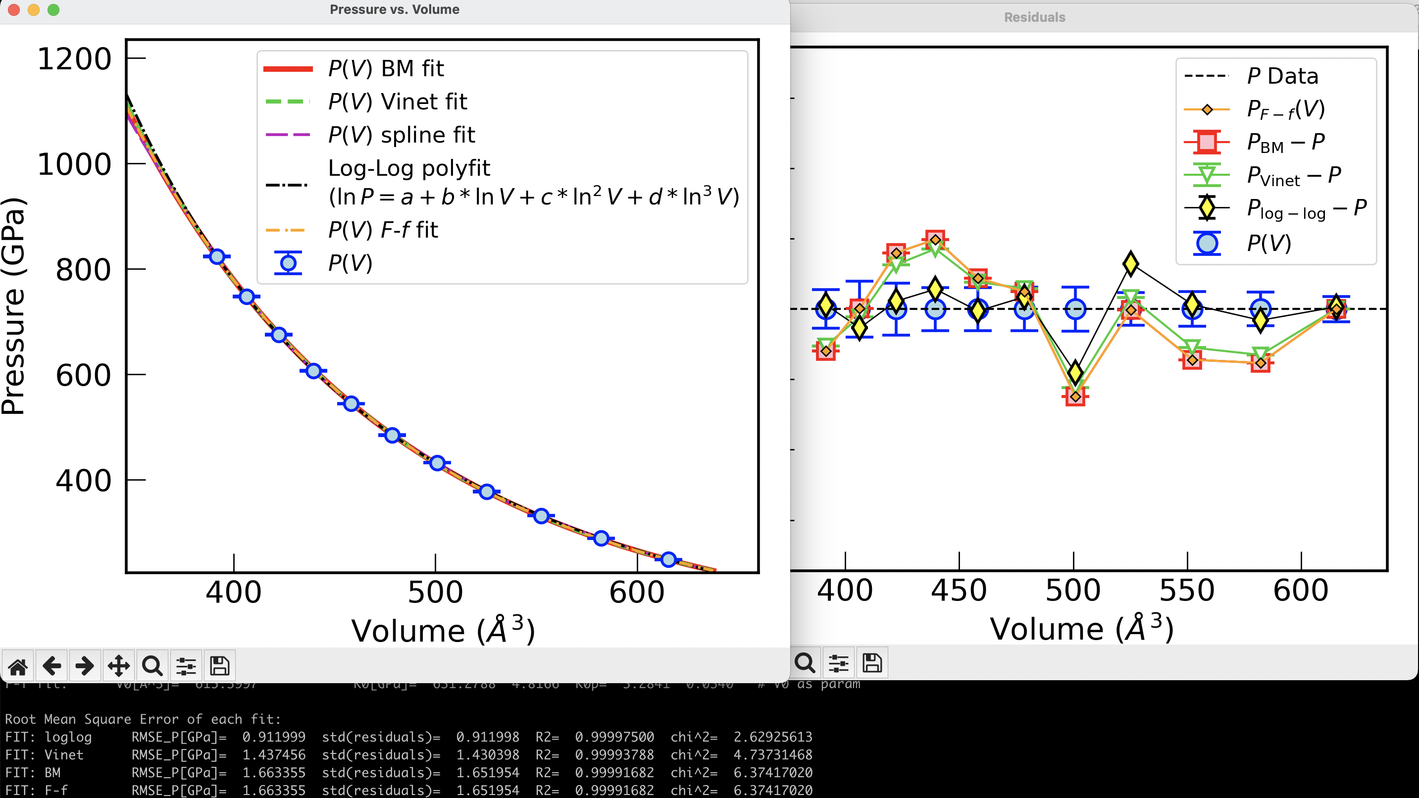
Two figures are generated by the code, using matplotlib: the original \(P\)-\(V\) data with errors together with all the fitting curves, and a figure with the differences \(P_{\rm fit}-P_{\rm data}\) (residuals) vs. volume. This provides a visual inspection of how far apart the predicted pressures are from the measured pressures. Compare this with the \(\chi^2\) diagnostics provided in the output.

Volume at \(P_{\text{Target}}\)

Adding a target pressure

./fit_EOS.py EOS_H2O_liq_7000K.dat 6 12 13 --PTarget 400.0 --noplots --BM4

Volume at P_Target
P_Target[GPa]=     400.00  V_BM[Å^3]=       514.7890 ± 0.7338
P_Target[GPa]=     400.00  V_F-f[Å^3]=      514.7890 ± 3.6574
P_Target[GPa]=     400.00  V_Vinet[Å^3]=    514.3874 ± 0.2865
P_Target[GPa]=     400.00  V_loglog[Å^3]=   514.8439 ± 332226.6620
P_Target[GPa]=     400.00  V_spline[Å^3]=   514.7242 ± 0.2578
PBest[GPa]=     377.5

\(\Delta G=\int_{P_1}^{P_{\rm Target}} V(P)dP = G(P_{\rm Target})- G(P_1)\)

As you can see above, providing the target pressure already provides the value of the integral for \(\Delta G\), but the default value is \(P_1= -1\) GPa. To change the value of \(P_1\), use --P1 and a value (integer or float) to the right:

./fit_EOS.py EOS_H2O_liq_7000K.dat 6 12 13 --PTarget 400.0 --P1 350 --BM4 

Volume at P_Target
P_Target[GPa]=     400.00  V_BM[Å^3]=       514.7890 ± 0.7338
P_Target[GPa]=     400.00  V_F-f[Å^3]=      514.7890 ± 3.6574
P_Target[GPa]=     400.00  V_Vinet[Å^3]=    514.3874 ± 0.2865
P_Target[GPa]=     400.00  V_loglog[Å^3]=   514.8439 ± 332226.6620
P_Target[GPa]=     400.00  V_spline[Å^3]=   514.7242 ± 0.2578
PBest[GPa]=     377.5
Integral from P1[GPa]=  -1.00 to P_Target[GPa]= 400.00:  ∆G[eV]= 1840.264831853906   ∆G[Ha]= 67.628485805681

The value of \(\Delta G\) is provided in eV, provided that \(P\) is in GPa and \(V\) is in ų.

Deleting points test: which fit performs better?

Using the --test option, the code will remove one point from the input dataset and refit the data. Since the removed point \((P_0,V_0)\) contains the known volume, the fit that better predicts \(V_0\) for fixed \(P_0\) is, in principle, the most reliable. A second round of tests removing two random datapoints from the dataset is performed in order to test the consistency:

./fit_EOS.py EOS_H2O_liq_7000K.dat 6 12 13  --noplots --test

**** FITTING EOS ****
by Felipe Gonzalez [Berkeley 05-19-2023]


#EOS Data: EOS_H2O_liq_7000K.dat
i=  0  V[A^3]=  615.3997  P[GPa]=  248.5530 0.4480
i=  1  V[A^3]=  582.1348  P[GPa]=  288.8810 0.5930
i=  2  V[A^3]=  552.2817  P[GPa]=  331.7850 0.6170
i=  3  V[A^3]=  525.3412  P[GPa]=  377.5250 0.5820
i=  4  V[A^3]=  500.9067  P[GPa]=  432.4520 0.7800
i=  5  V[A^3]=  478.6442  P[GPa]=  484.7840 0.7780
i=  6  V[A^3]=  458.2763  P[GPa]=  544.4000 0.7670
i=  7  V[A^3]=  439.5712  P[GPa]=  606.9460 0.7630
i=  8  V[A^3]=  422.3331  P[GPa]=  675.0050 0.9210
i=  9  V[A^3]=  406.3960  P[GPa]=  748.0080 0.9930
i= 10  V[A^3]=  391.6180  P[GPa]=  823.7650 0.6850
Birch-Murnaghan of degree 3

BM fit:       V0[A^3]=  615.3997            K0[GPa]=  631.2788  1.7987  K0p=  3.2841  0.0106   # Forcing P(V0)=P0 = min(P)
BM fit:       V0[A^3]= 1230.7993   13.6088  K0[GPa]=  101.5101  3.9648  K0p=  3.6423  0.0108   # V0 as param
Vinet fit:    V0[A^3]=  615.3997            K0[GPa]=  637.4325  2.2784  K0p=  3.2031  0.0197   # Forcing P(V0)=P0 = min(P)
Vinet fit:    V0[A^3]= 1846.1990  128.8517  K0[GPa]=   17.0905  5.2243  K0p=  5.3649  0.2220   # V0 as param

Root Mean Square Error of each fit:
FIT: BM         RMSE_P[GPa]=  1.663355  std(residuals)=  1.651954  R2=  0.99991682  chi^2=  6.37417020
FIT: Vinet      RMSE_P[GPa]=  1.437456  std(residuals)=  1.430398  R2=  0.99993788  chi^2=  4.73731468
FIT: loglog     RMSE_P[GPa]=  0.986809  std(residuals)=  0.986807  R2=  0.99997073  chi^2=  3.00585571

# DELETING POINTS TEST: removing one by one
P0[GPa]=   288.88  V0[A^3]=   582.13  V_BM[A^3]=   580.62  V_Vinet[A^3]=   580.83  V_loglog[A^3]=   581.95  V_BM_err[%]=  -0.260  V_Vinet_err[%]=  -0.223  V_loglog_err[%]=  -0.032
P0[GPa]=   331.79  V0[A^3]=   552.28  V_BM[A^3]=   551.05  V_Vinet[A^3]=   551.32  V_loglog[A^3]=   552.61  V_BM_err[%]=  -0.223  V_Vinet_err[%]=  -0.175  V_loglog_err[%]=   0.060
P0[GPa]=   377.52  V0[A^3]=   525.34  V_BM[A^3]=   525.32  V_Vinet[A^3]=   525.61  V_loglog[A^3]=   526.54  V_BM_err[%]=  -0.004  V_Vinet_err[%]=   0.051  V_loglog_err[%]=   0.229
P0[GPa]=   432.45  V0[A^3]=   500.91  V_BM[A^3]=   499.34  V_Vinet[A^3]=   499.48  V_loglog[A^3]=   499.46  V_BM_err[%]=  -0.313  V_Vinet_err[%]=  -0.285  V_loglog_err[%]=  -0.289
P0[GPa]=   484.78  V0[A^3]=   478.64  V_BM[A^3]=   478.92  V_Vinet[A^3]=   478.97  V_loglog[A^3]=   478.69  V_BM_err[%]=   0.058  V_Vinet_err[%]=   0.068  V_loglog_err[%]=   0.010
P0[GPa]=   544.40  V0[A^3]=   458.28  V_BM[A^3]=   458.70  V_Vinet[A^3]=   458.64  V_loglog[A^3]=   458.17  V_BM_err[%]=   0.091  V_Vinet_err[%]=   0.079  V_loglog_err[%]=  -0.024
P0[GPa]=   606.95  V0[A^3]=   439.57  V_BM[A^3]=   440.39  V_Vinet[A^3]=   440.26  V_loglog[A^3]=   439.90  V_BM_err[%]=   0.186  V_Vinet_err[%]=   0.158  V_loglog_err[%]=   0.076
P0[GPa]=   675.00  V0[A^3]=   422.33  V_BM[A^3]=   422.88  V_Vinet[A^3]=   422.76  V_loglog[A^3]=   422.59  V_BM_err[%]=   0.129  V_Vinet_err[%]=   0.101  V_loglog_err[%]=   0.061
P0[GPa]=   748.01  V0[A^3]=   406.40  V_BM[A^3]=   406.40  V_Vinet[A^3]=   406.33  V_loglog[A^3]=   406.33  V_BM_err[%]=   0.001  V_Vinet_err[%]=  -0.017  V_loglog_err[%]=  -0.015
P0[GPa]=   823.76  V0[A^3]=   391.62  V_BM[A^3]=   390.57  V_Vinet[A^3]=   390.84  V_loglog[A^3]=   391.23  V_BM_err[%]=  -0.268  V_Vinet_err[%]=  -0.200  V_loglog_err[%]=  -0.098
BEST SCORES:   {'BM': 2, 'Vinet': 1, 'loglog': 7} out of 10
WORST SCORES:  {'BM': 7, 'Vinet': 2, 'loglog': 1} out of 10
BEST FOR EXTRAPOLATIONS:   loglog
Overall scores: {'BM': -5, 'Vinet': -1, 'loglog': 6}
Best predictor: loglog

# DELETING TWO RANDOM POINTS TEST: (P0,V0) is one of them
P0[GPa]=   484.78  V0[A^3]=   478.64  V_BM[A^3]=   478.79  V_Vinet[A^3]=   478.86  V_loglog[A^3]=   478.73  V_BM_err[%]=   0.030  V_Vinet_err[%]=   0.044  V_loglog_err[%]=   0.018
P0[GPa]=   331.79  V0[A^3]=   552.28  V_BM[A^3]=   550.97  V_Vinet[A^3]=   551.23  V_loglog[A^3]=   552.59  V_BM_err[%]=  -0.237  V_Vinet_err[%]=  -0.191  V_loglog_err[%]=   0.055
P0[GPa]=   331.79  V0[A^3]=   552.28  V_BM[A^3]=   550.79  V_Vinet[A^3]=   551.04  V_loglog[A^3]=   552.18  V_BM_err[%]=  -0.269  V_Vinet_err[%]=  -0.225  V_loglog_err[%]=  -0.018
P0[GPa]=   675.00  V0[A^3]=   422.33  V_BM[A^3]=   423.03  V_Vinet[A^3]=   422.88  V_loglog[A^3]=   422.78  V_BM_err[%]=   0.164  V_Vinet_err[%]=   0.129  V_loglog_err[%]=   0.105
P0[GPa]=   544.40  V0[A^3]=   458.28  V_BM[A^3]=   458.92  V_Vinet[A^3]=   458.80  V_loglog[A^3]=   458.28  V_BM_err[%]=   0.140  V_Vinet_err[%]=   0.115  V_loglog_err[%]=   0.001
P0[GPa]=   675.00  V0[A^3]=   422.33  V_BM[A^3]=   422.91  V_Vinet[A^3]=   422.79  V_loglog[A^3]=   422.60  V_BM_err[%]=   0.136  V_Vinet_err[%]=   0.108  V_loglog_err[%]=   0.064
P0[GPa]=   331.79  V0[A^3]=   552.28  V_BM[A^3]=   550.79  V_Vinet[A^3]=   551.04  V_loglog[A^3]=   552.18  V_BM_err[%]=  -0.269  V_Vinet_err[%]=  -0.225  V_loglog_err[%]=  -0.018
P0[GPa]=   432.45  V0[A^3]=   500.91  V_BM[A^3]=   499.40  V_Vinet[A^3]=   499.52  V_loglog[A^3]=   499.46  V_BM_err[%]=  -0.300  V_Vinet_err[%]=  -0.276  V_loglog_err[%]=  -0.288
P0[GPa]=   606.95  V0[A^3]=   439.57  V_BM[A^3]=   440.40  V_Vinet[A^3]=   440.27  V_loglog[A^3]=   439.90  V_BM_err[%]=   0.189  V_Vinet_err[%]=   0.158  V_loglog_err[%]=   0.076
P0[GPa]=   331.79  V0[A^3]=   552.28  V_BM[A^3]=   550.79  V_Vinet[A^3]=   551.04  V_loglog[A^3]=   552.18  V_BM_err[%]=  -0.269  V_Vinet_err[%]=  -0.225  V_loglog_err[%]=  -0.018
P0[GPa]=   331.79  V0[A^3]=   552.28  V_BM[A^3]=   550.97  V_Vinet[A^3]=   551.23  V_loglog[A^3]=   552.59  V_BM_err[%]=  -0.237  V_Vinet_err[%]=  -0.191  V_loglog_err[%]=   0.055
P0[GPa]=   606.95  V0[A^3]=   439.57  V_BM[A^3]=   440.50  V_Vinet[A^3]=   440.35  V_loglog[A^3]=   439.90  V_BM_err[%]=   0.212  V_Vinet_err[%]=   0.176  V_loglog_err[%]=   0.076
P0[GPa]=   331.79  V0[A^3]=   552.28  V_BM[A^3]=   551.05  V_Vinet[A^3]=   551.32  V_loglog[A^3]=   552.62  V_BM_err[%]=  -0.223  V_Vinet_err[%]=  -0.174  V_loglog_err[%]=   0.061
P0[GPa]=   748.01  V0[A^3]=   406.40  V_BM[A^3]=   406.48  V_Vinet[A^3]=   406.39  V_loglog[A^3]=   406.41  V_BM_err[%]=   0.021  V_Vinet_err[%]=  -0.001  V_loglog_err[%]=   0.004
P0[GPa]=   748.01  V0[A^3]=   406.40  V_BM[A^3]=   406.40  V_Vinet[A^3]=   406.33  V_loglog[A^3]=   406.25  V_BM_err[%]=   0.001  V_Vinet_err[%]=  -0.017  V_loglog_err[%]=  -0.035
P0[GPa]=   331.79  V0[A^3]=   552.28  V_BM[A^3]=   550.97  V_Vinet[A^3]=   551.23  V_loglog[A^3]=   552.59  V_BM_err[%]=  -0.237  V_Vinet_err[%]=  -0.191  V_loglog_err[%]=   0.055
P0[GPa]=   331.79  V0[A^3]=   552.28  V_BM[A^3]=   551.19  V_Vinet[A^3]=   551.44  V_loglog[A^3]=   552.58  V_BM_err[%]=  -0.197  V_Vinet_err[%]=  -0.153  V_loglog_err[%]=   0.053
P0[GPa]=   331.79  V0[A^3]=   552.28  V_BM[A^3]=   551.02  V_Vinet[A^3]=   551.34  V_loglog[A^3]=   553.24  V_BM_err[%]=  -0.229  V_Vinet_err[%]=  -0.170  V_loglog_err[%]=   0.173
P0[GPa]=   675.00  V0[A^3]=   422.33  V_BM[A^3]=   422.86  V_Vinet[A^3]=   422.75  V_loglog[A^3]=   422.60  V_BM_err[%]=   0.125  V_Vinet_err[%]=   0.098  V_loglog_err[%]=   0.064
P0[GPa]=   675.00  V0[A^3]=   422.33  V_BM[A^3]=   422.84  V_Vinet[A^3]=   422.74  V_loglog[A^3]=   422.55  V_BM_err[%]=   0.121  V_Vinet_err[%]=   0.096  V_loglog_err[%]=   0.053
BEST SCORES:   {'BM': 1, 'Vinet': 3, 'loglog': 16} out of 20
WORST SCORES:  {'BM': 18, 'Vinet': 1, 'loglog': 1} out of 20
Overall scores: {'BM': -17, 'Vinet': 2, 'loglog': 15}
Best predictor two-points test: loglog

Merge plots

We can merge the \(P(V)\) plot with the plot of the residuals using the --merge-plots option.

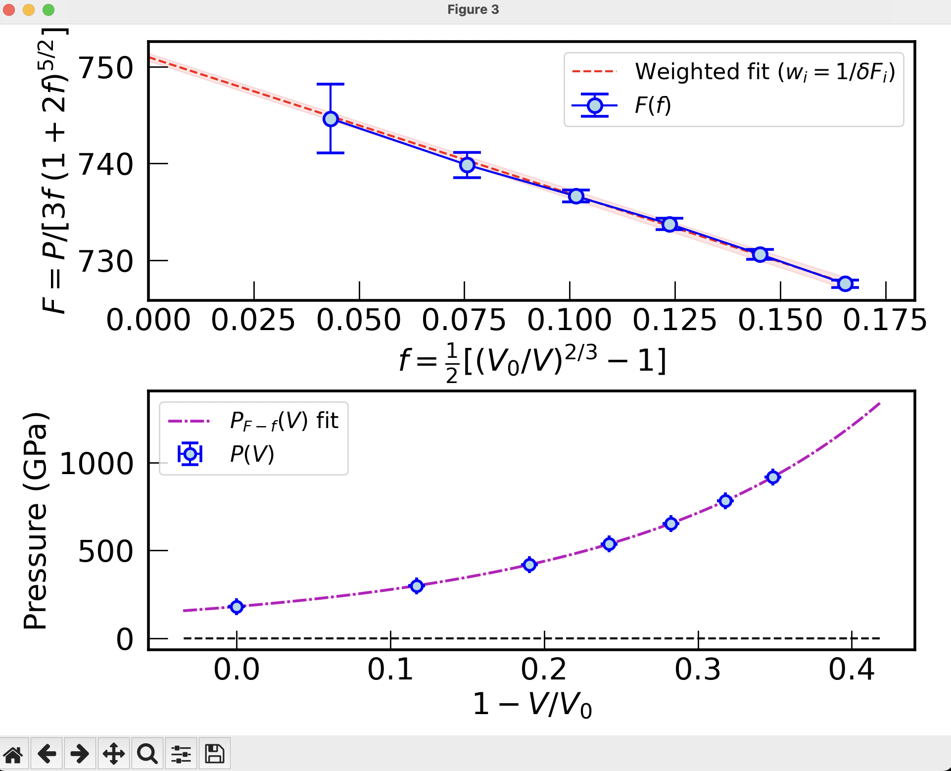
The \(F\) vs. \(f\) plot

In addition, we can display the optional plot of \(F\) vs. \(f\) plot using the --show-F-plot. A weighted linear interpolation of \(F-f\) is equivalent to a third-order Birch-Murnaghan. A positive slope of \(F(f)\) means that \(K_0'>4\):

./fit_EOS.py EOS_Au_sol_298K.dat 5 7 2 4  --merge-plots  --show-F-plot

Output

BM fit:       V0[A^3]=    0.9759            K0[GPa]=  186.8480  5.4645  K0p=  5.3998  0.3833   # Forcing P(V0)=P0 = min(P)
BM fit:       V0[A^3]=    0.9901    0.0005  K0[GPa]=  255.3038  7.8136  K0p=  1.9907  0.2382   # V0 as param
Vinet fit:    V0[A^3]=    0.9759            K0[GPa]=  186.6511  5.3937  K0p=  5.5409  0.3662   # Forcing P(V0)=P0 = min(P)
Vinet fit:    V0[A^3]=    0.9894    0.0006  K0[GPa]=  266.7909  9.3964  K0p=  1.1654  0.3807   # V0 as param
F-f fit:      V0[A^3]=    1.0000            K0[GPa]=  166.5037  9.1082  K0p=  2.5854  0.6648

Root Mean Square Error of each fit:
FIT: F-f        RMSE_P[GPa]=  1.367572  std(residuals)=  1.233342  R2=  0.99568453  chi^2=  33.16240413
FIT: Vinet      RMSE_P[GPa]=  1.366368  std(residuals)=  1.207360  R2=  0.99569212  chi^2=  38.02242777
FIT: BM         RMSE_P[GPa]=  1.380015  std(residuals)=  1.218643  R2=  0.99560564  chi^2=  38.13478882
FIT: loglog     RMSE_P[GPa]=  1.044243  std(residuals)=  1.044211  R2=  0.99748388  chi^2=  140.47121731